Volumetric in ArcMap

Intro:

Volumetric analysis is a simple skill that is invaluable because it separates the pros from the average data collector. It is also something that can ruin your reputation if you are bad at it because surveyors will run their own data and find the discrepancies in your data.

Methods:
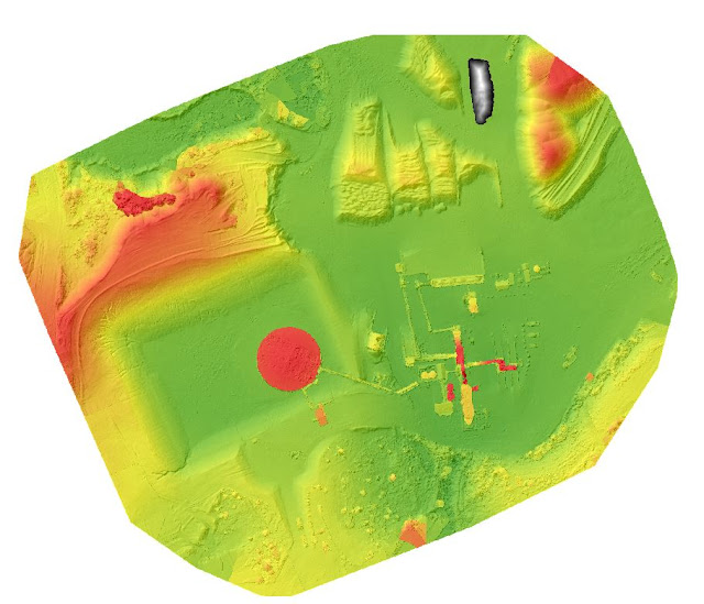
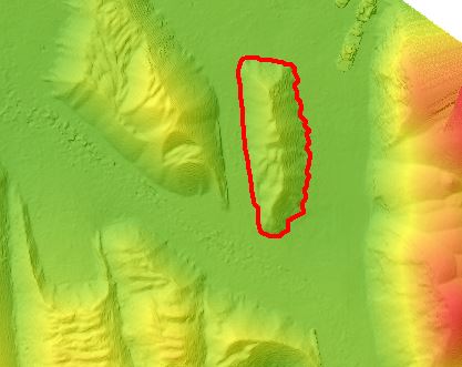
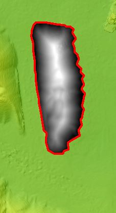
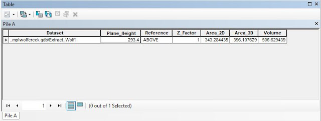
I used ArcMap to find the volume of a pile and the entire mine. I pulled up the DSM and Hillshade from the Wolfcreek mine. The first step is to clip the image around the pile I wanted to measure. It is important to make this as accurate as possible so there is little to no skewed data. Next I used "Extract by Mask" to make the cookie cutter image of the pile. Then i used the "Identify" tool to find the base level. Then I used "Surface Volume"  where I put in the base level and had it find the data above the base level. After this the data from the file will be shown. Figures 1-4.

To demonstrate the Cut-Fill for Litchfield I used ArcMap as well. I used Images collected on 07/22/2017 and 09/30/2017. I transferred the DSM of both images over to ArcMap. The first step is to use the "Resample" tool to make the images move from sub-millimeter accuracy to 10 centimeter accuracy. this enlarges the pixels because we don't need every little divot in the pile, and it will also save us a lot of time while analyzing the data. Then use the "Cut-Fill" tool and input the first image (07/22/2017) in the first raster data set then the second image (09/30/2017) in the second raster data set. This makes the data compare where the material is in the first image (07/22/2017) to where the material is in the second image (09/30/2017). Figure 5-7.

Discussion:

You can follow the steps from above to figures 1-4 below to get a better view of what I did to collect the data. A lot of what I did in this post is very similar or exactly what I did in the "Open Source GIS and Volumetrics" post right before this post.

Figure 1: Shows the full Orthomosaic of the Wolfcreek mine with. The blacked out area in the top right corner is the pile I did the analysis on.

Figure 2: This is where I plotted my line out around the pile to create the cookie cutter layer of the image.

Figure 3: This is where I found my base level to input into the surface volume tool to find the volume of everything above this level.

Figure 4: This is the data I received after. This is the final product that you will need to turn into your clients unless the want the weight of the pile, I will go over how to find that out in the next step. The base level is the height that the software calculated everything above in the blacked out section (293.4 m). The Grid Volume is the actual volume of the actual pile (506.629439 cubic meters).

Figure 1

Figure 2

Figure 3

Figure 4

For the Cut-Fill of the Litchfield mine the images are below Figures 5-7.

With Figure 7 the Red area is where material was gained, the Blue area is where material was lost, and the Grey area is where material stayed the same. As you can see there is no grey area because every space was change even the slightest. I could have changed the amount of material change to allow for more grey to show up, but I wanted to show how no matter what in an uncontrollable environment everything will be effected even if it is only by a few millimeters. I can easily change this to conform to a clients specific wants and needs.

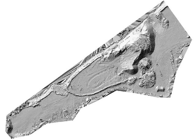Figure5  (07/22/2017)

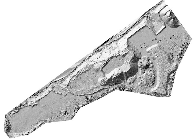Figure 6 (09/30/2017)

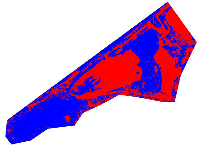Figure 7

Conclusion: 

I have proven that I have the abilities and knowledge to find the volume of a smaller area such as the pile in Figures 1-3 and larger areas in Figures 5-7. These are skills that will put me above the rest of the people in my career field.